Policy search is a crucial aspect in Reinforcement Learning as it directly relates to the optimization of the algorithm in weight space. Various environments are used for benchmarking policy search including the famous ATARI 2600 games and MuJoCo control suite. However, various environments have longer horizons which force the agent to perform better at continuous timesteps. This is often a non-trivial problem when dealing with policy-based approaches. This post introduces a new environment called the CyclicMDP which is a long horizon discrete problem presented to the agent. The environment is competitive to modern-day RL benchmarks is the sense that it presents the agent with a simple problem but at a very long (ideally infinite) horizon.

The CyclicMDP

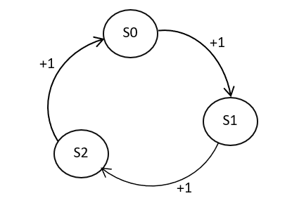
The CyclicMDP consists of 3 states and 3 actions. The agent starts in state S0 and has 3 actions- Move Left, Move Right and Stay. The state S0 is connected to S1 on the left and S2 on the right. The state S1 is connected to S2 on the left and S0 on the right and state S2 is connected to S0 on the left and S1 on the right. The agent is presented with the objective to go left at each timestep. A reward of +1 is presented to the agent if it goes left and 0 for any other action. Although, the environment does not have a horizon end to it, reward values of 1000, 5000 or 10000 are suitable to make it a long horizon problem.

The MDP is designed to study and analyze the underlying decision-making aspects of policy-based algorithms such as A2C, DDPG and PPO. These algorithms, making use of an Actor-Critic setup, search for optimal policies by directly applying the changes to it. The Actor-Critic setup makes use of Advantage estimates which can often be noisy in the sense that state values tend to changes quite often. This leads to significant deviation and high variance in the updates. CyclicMDP, having a small state-space and action-space, poses a long-horizon objective to the agent which can lead to noisy estimates and different inferences of the same result.

The Environment Design

We construct the CyclicMDP in Python by only making the use of the `numpy` library. The environment, just like any other environment, has 3 parts to it- `init`, `step` and `reset` methods. So lets have a look at these-

import numpy as np

class CyclicMDP:
    def __init__(self):
        self.end           = False
        self.current_state = 1
        self.num_actions   = 3
        self.num_states    = 3

We initialize `num_states` as the number of states, `nu_actions` as the number of actions, `end` as a signal which indicates termination of the episode and `current_state` as the state from which the agent begins.

def reset(self):
        self.end = False
        self.current_state = 1
        state = np.zeros(self.num_states)
        state[self.current_state - 1] = 1.
        return state

The `reset` method sets the environment back to its initial state upon the beginning of an episode. The agent starts in state S0 which is hot-one encoded for the agent.

 def step(self, action):
        if self.current_state == 1 or self.current_state == 2:
            if action == 1:
                    self.current_state += 1
                    reward = 1
                    
            else:
                reward = -1
                self.end = True

        else:
            if action == 1:
                    self.current_state = 1
                    reward = 2
                    
            else:
                reward = -1
                self.end = True
	    
        state = np.zeros(self.num_states)
        state[self.current_state - 1] = 1
        return state, reward, self.end, {}

The `step` function consists of action execution and state transitions. Once the agent performs its action, the state `current_state` transitions to the next state and the agent observes the reward `reward`.

Agent Behavior

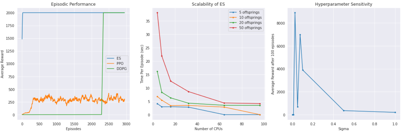
CyclicMDP results have mixed performance for various algorithms. In the case of [PPO](https://arxiv.org/pdf/1707.06347.pdf), the agent gets stuck on a local optima early in training as a result of proximal policy search. This can be interpreted as a difficult problem for the agent since it is only searching specific regions of the weight space as it is contrained to the trust region. On the other hand, Evolution Strategies [(ES)](https://openai.com/blog/evolution-strategies/), a genetic algorithm which will be discussed in future posts, performs significantly well. Primary reason behind this finding is that ES does not make use of backpropagation updates and uses multiple models as its agents to traverse through the weight space. The probability of ES finding the long-sighted global convergence is much higher in comparison to Policy Gradient methods.

In terms of scalability, CyclicMDP is parallelizable as it has small runtime per episode. Complex algorithms such as ES making use of multiple models in its population can be easily scaled up using parallel compute.

Another notable finding is that CyclicMDP presents a good benchmark for hyperparameter analysis. Sigma being a tricky parameter for ES can be tuned with ease given domain-specific knowledge of the algorithm.

Limitations

Although CyclicMDP is a versatile and easy-to-use environment, it lacks certain features which modern-day algorithms pose as a challenging task. These are as followed-

1. CyclicMDP has a small action space and fails to address the open problem of larger action spaces.
2. Being a discrete environment, CyclicMDP cannot replicate continuous and dynamically controlling nature of the agent.
3. Given the infinite horizon case, the environment can get stuck and may never lead to the termination of an episode. In such cases, a timeout may be used which would allow the agent to play an episode only for a fixed duration of time.